Some intermediate DB2 SQL techniques
Set up tables, logicals, labels and add some dataUse SQL Join to combine Headers and Details
Types of Joins
Example of a full OUTER JOIN
Subquery vs Common Table Expression
Use a subquery and RRN() function to identify and delete duplicate data
Update using a subselect in the WHERE clause
The Case Statement
Find gaps in order file using OLAP Lead() and Lag() functions:
Calculating rank with OLAP Rank() and Over() functions
Using HAVING to filter on GROUP BY values
Use SQL Hierarchical Query Operators PRIOR and CONNECT_BY_ROOT
SQL Stored Procedures
Set up tables, logicals, labels and add some data
Here we will take a look at some interesting SQL techniques. Note that some syntax may be specific to DB2 or DB2 for iSeries..., but first let's create some tables and set up some data.
Create a Customer Master table
CREATE TABLE MYLIB/CUSTOMER (
  CUST_CODE INT NOT NULL WITH DEFAULT,
  CUST_TYPE CHAR (1) NOT NULL WITH DEFAULT,
  CUST_NAME CHAR (25) NOT NULL WITH DEFAULT,
  CUST_ADDRESS CHAR (25) NOT NULL WITH DEFAULT,
  CUST_YR_SALES INT NOT NULL WITH DEFAULT
)
RCDFMT CUSTOMERR
Create an Order Header table
CREATE TABLE MYLIB/ORDER_HED (
  ORDER_NUM INT NOT NULL WITH DEFAULT,
  ORDER_CUST INT NOT NULL WITH DEFAULT,
  ORDER_DATE DATE NOT NULL WITH DEFAULT,
  ORDER_TIME TIME NOT NULL WITH DEFAULT,
  ORDER_VALUE DEC ( 11, 2) NOT NULL WITH DEFAULT
)
RCDFMT  ORDER_HEDR
Create an Order Detail table
CREATE TABLE MYLIB/ORDER_DET (
    DETAIL_NUM INT NOT NULL WITH DEFAULT,
    DETAIL_LIN INT NOT NULL WITH DEFAULT,
    DETAIL_SKU CHAR (25) NOT NULL WITH DEFAULT,
    DETAIL_QTY INT NOT NULL WITH DEFAULT,
    DETAIL_PRI DEC ( 10, 2) NOT NULL WITH DEFAULT
 )
 RCDFMT  ORDER_DETR
Add an index
 CREATE INDEX MYLIB/ORD_DETL1
    ON ORDER_DET(DETAIL_NUM, DETAIL_LIN)
Give descriptions to table and index
LABEL ON TABLE MYLIB/ORDER_DET
IS 'Order Detail'

LABEL ON INDEX MYLIB/ORD_DETL1
IS 'Order Header -index'
Add some column labels
LABEL ON COLUMN ORDER_HED
(  ORDER_NUM   TEXT IS 'Order_Number',
   ORDER_CUST  TEXT IS 'Order_Customer',
   ORDER_DATE  TEXT IS 'Order_Date',
   ORDER_TIME  TEXT IS 'Order_Time',
   ORDER_VALUE TEXT IS 'Order Value')

LABEL ON COLUMN ORDER_DET
(  DETAIL_NUM    TEXT IS 'Order_Number',
   DETAIL_LIN   TEXT IS 'Line_Number',
   DETAIL_SKU    TEXT IS 'SKU',
   DETAIL_QTY    TEXT IS 'Quantity',
   DETAIL_PRI  TEXT IS 'Price'
)
Add add some data
INSERT INTO CUSTOMER VALUES('10001','A', 'Reliable Rug Cleaning', '124 Main Street', 300)
INSERT INTO CUSTOMER VALUES('10003','A', 'Circle K', '125 Main Street', 200)
INSERT INTO CUSTOMER VALUES('10005','A', 'St Hubert BAR-B-Q', '126 Main Street', 100)
INSERT INTO CUSTOMER VALUES('10006','B', 'Patisserie Polonaiss', '127 Main Street', 150)
INSERT INTO CUSTOMER VALUES('10007','B', 'Kintuky Fried Chickun', '128 Main Street', 250)
INSERT INTO CUSTOMER VALUES('10008','B', 'Brasserie Nuit Blanc', '129 Main Street', 350)
INSERT INTO CUSTOMER VALUES('10009','C', 'La Tienda', '130 Main Street', 400)
INSERT INTO CUSTOMER VALUES('10010','C', 'IGA', '131 Main Street', 200)
INSERT INTO CUSTOMER VALUES('10011','C', 'RGB Indian Food', '132 Main Street', 600)


INSERT INTO ORDER_HED VALUES(100, '10001', '01/13/2016', '12:00:01',  110)
INSERT INTO ORDER_HED VALUES(101, '10003', '02/14/2016', '12:00:02',  120)
INSERT INTO ORDER_HED VALUES(102, '10006', '04/15/2016', '12:00:03',  130)
INSERT INTO ORDER_HED VALUES(105, '10007', '05/13/2016', '12:00:01',  140)
INSERT INTO ORDER_HED VALUES(106, '10001', '05/13/2016', '12:00:01',  150)
INSERT INTO ORDER_HED VALUES(110, '10003', '07/14/2016', '12:00:02',  160)
INSERT INTO ORDER_HED VALUES(112, '10006', '09/15/2016','12:00:03',  170)
INSERT INTO ORDER_HED VALUES(113, '10007', '12/13/2016', '12:00:01',  180)

INSERT INTO ORDER_DET VALUES(100, 1, 'ABCD12345678901234567890', 1, 50.00)
INSERT INTO ORDER_DET VALUES(100, 2, 'ABCD12345678901234567891', 1, 60.00)
INSERT INTO ORDER_DET VALUES(101, 1, 'ABCD12345678901234567892', 1, 50.00)
INSERT INTO ORDER_DET VALUES(101, 2, 'ABCD12345678901234567893', 1, 70.00)
INSERT INTO ORDER_DET VALUES(102, 1, 'ABCD12345678901234567894', 1, 50.00)
INSERT INTO ORDER_DET VALUES(102, 2, 'ABCD12345678901234567895', 1, 80.00)
INSERT INTO ORDER_DET VALUES(105, 1, 'ABCD12345678901234567896', 1, 50.00)
INSERT INTO ORDER_DET VALUES(105, 2, 'ABCD12345678901234567897', 1, 90.00)
INSERT INTO ORDER_DET VALUES(106, 1, 'ABCD12345678901234567898', 1, 50.00)
INSERT INTO ORDER_DET VALUES(106, 2, 'ABCD12345678901234567899', 1, 100.00)
INSERT INTO ORDER_DET VALUES(110, 1, 'ABCD12345678901234567900', 1, 50.00)
INSERT INTO ORDER_DET VALUES(110, 2, 'ABCD12345678901234567901', 1, 110.00)
INSERT INTO ORDER_DET VALUES(112, 1, 'ABCD12345678901234567902', 1, 50.00)
INSERT INTO ORDER_DET VALUES(112, 2, 'ABCD12345678901234567903', 1, 120.00)
INSERT INTO ORDER_DET VALUES(113, 1, 'ABCD12345678901234567904', 1, 50.00)
INSERT INTO ORDER_DET VALUES(113, 2, 'ABCD12345678901234567905', 1, 130.00)
Use SQL Join to combine Headers and Details
A JOIN clause is used to combine rows from two or more tables, based on a related column between them.
SELECT ORDER_HED.ORDER_NUM, ORDER_DET.DETAIL_LIN,
    ORDER_DET.DETAIL_SKU, ORDER_DET.DETAIL_QTY, ORDER_DET.DETAIL_PRI,
	ORDER_DET.DETAIL_QTY * ORDER_DET.DETAIL_PRI as TOTAL
FROM ORDER_HED JOIN ORDER_DET ON (ORDER_HED.ORDER_NUM = ORDER_DET.DETAIL_NUM )
Note that we can also use the WHERE clause instead of JOIN ON clause.
SELECT ORDER_HED.ORDER_NUM, ORDER_DET.DETAIL_LIN,
    ORDER_DET.DETAIL_SKU, ORDER_DET.DETAIL_QTY, ORDER_DET.DETAIL_PRI,
	ORDER_DET.DETAIL_QTY * ORDER_DET.DETAIL_PRI  as TOTAL
FROM ORDER_HED , ORDER_DET
WHERE ORDER_HED.ORDER_NUM = ORDER_DET.DETAIL_NUM
Output:
ORDER_NUM     DETAIL_LIN   DETAIL_SKU     DETAIL_QTY    DETAIL_PRI                          TOTAL
       100               1   ABCD                    1           50,00                          50,00
       100               2   ABCD                    1           60,00                          60,00
       101               1   ABCD                    1           50,00                          50,00
       101               2   ABCD                    1           70,00                          70,00
       102               1   ABCD                    1           50,00                          50,00
       102               2   ABCD                    1           80,00                          80,00
       105               1   ABCD                    1           50,00                          50,00
       105               2   ABCD                    1           90,00                          90,00
...
 ********  End of data  ********
Types of Joins and Union
JOIN or INNER JOIN - An Inner join is a method of combining two tables that discard rows of either table that do not match any row of the other table. The matching is based on the join condition.
LEFT JOIN or LEFT OUTER JOIN - A left outer join is a method of combining tables. The result includes unmatched rows from only the table that is specified before the LEFT OUTER JOIN clause.
RIGHT JOIN or RIGHT OUTER JOIN - A right outer join is a method of combining tables. The result includes unmatched rows from only the table that is specified after the RIGHT OUTER JOIN clause.
FULL OUTER JOIN - A full outer join is a method of combining tables so that the result includes unmatched rows of both tables.
UNION - allows you to combine results of two or more SELECT statements into a single result set which includes all the rows that belong to the SELECT statements in the union. Each SELECT statement within UNION must have the same number of columns. The columns must also have similar data types. The columns in each SELECT statement must also be in the same order.
Example of a FULL OUTER JOIN
The FULL OUTER JOIN allows you to combine tables so that the result includes both matched and unmatched rows of both tables. To test the FULL OUTER JOIN, let's insert "orphan" header and footer records into the database, then use the FULL OUTER JOIN to catch all matches and non-matched records.
INSERT INTO ORDER_HED VALUES(777, '10005', '01/13/2016','12:00:03', 0)
INSERT INTO ORDER_DET VALUES(888, 2, 'SHES', 2, 13.99)
SELECT ORDER_HED.ORDER_NUM, ORDER_DET.DETAIL_LIN,
   ORDER_DET.DETAIL_SKU, ORDER_DET.DETAIL_QTY, ORDER_DET.DETAIL_PRI,
   ORDER_DET.DETAIL_QTY * ORDER_DET.DETAIL_PRI as TOTAL
FROM ORDER_HED FULL OUTER JOIN ORDER_DET
   ON (ORDER_HED.ORDER_NUM = ORDER_DET.DETAIL_NUM )
Note the dashes representing null values in the results below, where the SQL query does not find matches using a FULL OUTER JOIN.
ORDER_NUM     DETAIL_LIN   DETAIL_SKU     DETAIL_QTY    DETAIL_PRI                          TOTAL
       112               1   ABCD                    1           50,00                          50,00
       112               2   ABCD                    1          120,00                         120,00
       113               1   ABCD                    1           50,00                          50,00
       113               2   ABCD                    1          130,00                         130,00
       777                -  -                        -               -                              -
          -              2   SHES                    2           13,99                          27,98
...
 ********  End of data  ********
The Subquery vs Common Table Expression (CTE)
A SQL subquery is a query inside a query. A subquery is also called a nested query or an inner query. The outer query in which the inner query is inserted is the main query. We can use it in multiple ways: in the FROM clause, for filtering, or even as a column.
The Common Table Expression (CTE) is a construct in SQL that helps simplify a query. CTEs work as virtual tables (with records and columns), created during the execution of a query, used by the query, and eliminated after query execution. CTEs often act as a bridge to transform the data in source tables to the format expected by the query.
Common table expression (CTE) vs subquery
| Criteria | Subquery | CTE | |
|---|---|---|---|
| Where defined | defined inline | at the front of the query | |
| naming | doesn't have a name | must always be named | |
| Can be used recursively | No | Yes | |
| Readable | Yes | Better | |
| Can be used many times within a query | Only once | Yes | |
| Can be used within WHERE clause in conjunction with the keywords IN or EXISTS | No | Yes | |
| Can pick up a multiple pieces of data from one table in order to update a value in another table. | No. Only one value | Yes. Multiple Values | |
| Example 1: With list of Orders found in Order Detail file, check order value in Order Header file |
  SELECT
  ORDER_NUM, ORDER_VALUE
  FROM ORDER_HED

WHERE ORDER_NUM IN
  (
   SELECT DETAIL_NUM
   FROM ORDER_DET
   GROUP BY DETAIL_NUM
)
|
WITH MY_CTE AS ( SELECT DETAIL_NUM FROM ORDER_DET GROUP BY DETAIL_NUM ) SELECT ORDER_NUM, ORDER_VALUE FROM ORDER_HED JOIN MY_CTE ON (ORDER_NUM = DETAIL_NUM ) |
|
| Example 2 |
N/A |
WITH MY_CTE AS (
   SELECT DETAIL_NUM,
   sum(DETAIL_QTY* DETAIL_PRI) AS SUM_OF_DET
   FROM ORDER_DET
   GROUP BY DETAIL_NUM
)
SELECT  DETAIL_NUM, ORDER_VALUE, MY_CTE.SUM_OF_DET
    FROM ORDER_HED JOIN MY_CTE
    ON (MY_CTE.DETAIL_NUM = ORDER_HED.ORDER_NUM)
|
Multiple Subqueries in a single SQL statement
Show orders and how many units in the order and the average number of units for all orders.
SELECT DETAIL_NUM AS ORDER_NO,
SUM( DETAIL_QTY ) AS UNITS_IN_ORDER,
(
	SELECT SUM(DETAIL_QTY)
	FROM ORDER_DET
	)
	/
	(SELECT CAST(COUNT(*) AS DECIMAL(9,2))
	FROM ORDER_HED
) AS AVG_UNITS_PER_ORDER
FROM ORDER_DET
GROUP BY DETAIL_NUM
ORDER BY DETAIL_NUM
ORDER_NO   UNITS_IN_ORDER   AVG_UNITS_PER_ORDER
        100                2                  2
        101                2                  2
        102                2                  2
        105                2                  2
...
********  End of data  ********
Update using a subselect in the WHERE clause
In this query we use a subquery to give 20% discount to customers who ordered before January 14th.
UPDATE  ORDER_DET SET DETAIL_PRI = DETAIL_PRI * .8
WHERE   ORDER_DET.DETAIL_NUM IN (
        SELECT   ORDER_NUM
        FROM     ORDER_HED
        WHERE    ORDER_DATE > '01/14/2016'
		)
Use a subquery and RRN function to identify and delete duplicate data.
The RRN function returns the relative record number of a row.
Say we have a customer code entered twice and we want to delete the second instance of the customer.
First we create a duplicate record:
INSERT INTO CUSTOMER VALUES('10001','A', 'BOB''S BAR-B-Q', '124 Main Street', 300)
Then identify duplicate record(s):
SELECT * from CUSTOMER E1
where RRN(E1) > (Select MIN(RRN(E2))
from CUSTOMER E2 where E2.CUST_CODE  = E1.CUST_CODE)
Next we can delete latest duplicate record:
Delete from CUSTOMER E1
where RRN(E1) > (Select MIN(RRN(E2)) from CUSTOMER E2 where E2.CUST_CODE = E1.CUST_CODE)
Or the earliest duplicate record:
Delete from CUSTOMER E1
where RRN(E1) < (Select MAX(RRN(E2)) from CUSTOMER E2 where E2.CUST_CODE = E1.CUST_CODE)
Or multiple records where there are multiple duplicates
DELETE from CUSTOMER E1 where RRN(E1) in (
  SELECT RRN(E2) from CUSTOMER E2 where RRN(E2) < (Select
MAX(RRN(E3)) from CUSTOMER E3 where E3.CUST_CODE = E2.CUST_CODE))
FETCH FIRST 2 ROWS ONLY
The Case Statement
The CASE statement goes through conditions and returns a value when the first condition is met (like an IF-THEN-ELSE statement). So, once a condition is true, it will stop reading and return the result. If no conditions are true, it returns the value in the ELSE clause. If there is no ELSE part and no conditions are true, it returns NULL. We can use a Case statement in select queries along with Where, Order By and Group By clause. It can be used in Insert statement as well.
Here we want to do tests on each order and add a comment for each based on order quantity.
SELECT ORDER_HED.ORDER_NUM,
    SUM(ORDER_DET.DETAIL_QTY) AS ORDER_QTY,
    CASE
       WHEN SUM(ORDER_DET.DETAIL_QTY) <= 3 THEN 'Small Order (3 units or less)'
       WHEN SUM(ORDER_DET.DETAIL_QTY) BETWEEN 4 and 5 THEN 'Medium Order (4 or 5 units)'
       ELSE 'Large Order (6 or more units)'
    END AS ORDER_COMMENT
 FROM ORDER_HED JOIN ORDER_DET
 ON(ORDER_HED.ORDER_NUM = ORDER_DET.DETAIL_NUM)
 GROUP BY ORDER_HED.ORDER_NUM
    ORDER_NUM       ORDER_QTY   ORDER_COMMENT
          100               3   Small Order (3 units or less)
          101               5   Medium Order (4 or 5 units)
          102               6   Large Order (6 or more units)
********  End of data  ********
Find gaps in order file using OLAP Lead() and Lag() functions:
The and Lead() and Lag() functions allow you to extract a column value from a different row within the result set (relative to the current row) without programmatically looping through each row. Here we use them to identify places with gaps in order number and report out GAP or no GAP using case statement.
SELECT
  ORDER_NUM,
  LAG(ORDER_NUM) OVER (ORDER BY ORDER_NUM) ,
  LEAD(ORDER_NUM) OVER (ORDER BY ORDER_NUM),
  CASE
    WHEN LAG(ORDER_NUM) OVER (ORDER BY ORDER_NUM) + 1 != ORDER_NUM
    THEN
      'GAP'
    ELSE
     'NO GAP'
    END AS Gap_Found
FROM ORDER_HED
output:
   ORDER_NUM             LAG            LEAD   GAP_FOUND
         100                -            101    NO GAP
         101             100             102    NO GAP
         102             101             105    NO GAP
         105             102             106    GAP
...
Find lowest and highest order number in Order Header files:
SELECT MIN(ORDER_NUM), MAX(ORDER_NUM) FROM ORDER_HED
Find specific order numbers missing in a sequence between lowest and highest order number in Order Header files:
 WITH A(NUM) AS
 (
  VALUES (SELECT MIN(ORDER_NUM) FROM ORDER_HED)
  UNION ALL
    SELECT NUM + 1
    FROM A
    WHERE Num < (SELECT MAX(ORDER_NUM) FROM ORDER_HED)
 )
 SELECT NUM FROM A WHERE Num not in (Select ORDER_NUM from
ORDER_HED)
output:
NUM
       103
       104
       107
       108
       109
       111
Calculating Rank with OLAP Rank() and Over() functions
The RANK() function is a window function that assigns a rank to each row in the partition of a result set. The rank of a row is determined by one plus the number of ranks that come before it.
The OVER() function is used in conjunction with a function like RANK or AVG The OVER keyword instructs DB2 to calculate the rank (or other function) over a range of values.
In example below, we rank by CUST_YR_SALES. If we have a tie, a rank may be shared by multiple customer, and then the next rank value is skipped
SELECT RANK() OVER (ORDER BY CUST_YR_SALES DESC)  AS RANK,
CUST_CODE,  CUST_YR_SALES
FROM CUSTOMER
ORDER BY CUST_YR_SALES DESC

 RANK       CUST_CODE   CUST_YR_SALES
    1          10.011             600
    2          10.009             400
    3          10.008             350
    4          10.001             300
    5          10.007             250
    6          10.003             200
    6          10.010             200
    8          10.006             150
    9          10.005             100
OLAP functions DENSE_RANK() and ROW_NUMBER()
If we use DENSE_RANK() we do not skip a ranking value in case of a tie.
SELECT DENSE_RANK() OVER (ORDER BY CUST_YR_SALES DESC)  AS RANK,
CUST_CODE,  CUST_YR_SALES
FROM CUSTOMER
ORDER BY CUST_YR_SALES DESC

RANK       CUST_CODE   CUST_YR_SALES
     1          10.011             600
     2          10.009             400
     3          10.008             350
     4          10.001             300
     5          10.007             250
     6          10.003             200
     6          10.010             200
     7          10.006             150
     8          10.005             100
ROW NUMBER() provides us with a row number. This can be useful feature when downloading file.
SELECT ROW_NUMBER() OVER (ORDER BY CUST_YR_SALES DESC)  AS ROW_NUMBER,
CUST_CODE,  CUST_YR_SALES
FROM CUSTOMER
ORDER BY CUST_YR_SALES DESC


ROW_NUMBER       CUST_CODE   CUST_YR_SALES
          1          10.011             600
          2          10.009             400
          3          10.008             350
          4          10.001             300
          5          10.007             250
          6          10.010             200
          7          10.003             200
          8          10.006             150
          9          10.005             100
Calculating Rank with OLAP Rank() and Over() functions and Partition By clause
Here we add additional the PARTITION BY clause
The PARTITION BY clause defines the partition within which the function is applied. A partitioning-expression is an expression that is used in defining the partitioning of the result set.
This example gives us rank top customers by sales partitioned by customer type
SELECT RANK() OVER (PARTITION BY CUST_TYPE
                    ORDER BY CUST_YR_SALES DESC)  AS RANK,
CUST_TYPE, CUST_CODE,  CUST_YR_SALES
FROM CUSTOMER
ORDER BY CUST_TYPE, CUST_YR_SALES DESC


RANK   CUST_TYPE      CUST_CODE   CUST_YR_SALES
    1       A             10.001             300
    2       A             10.003             200
    3       A             10.005             100
    1       B             10.008             350
    2       B             10.007             250
    3       B             10.006             150
    1       C             10.011             600
    2       C             10.009             400
    3       C             10.010             200
Using HAVING to filter on GROUP BY values
The HAVING clause enables you to specify conditions that filter which group results appear in the final results. The WHERE clause places conditions on the selected columns, whereas the HAVING clause places conditions on groups created by the GROUP BY clause. In this example, we use HAVING and GROUP BY to show orders whose total is greater than $50
SELECT    ORDER_HED.ORDER_NUM, SUM( ORDER_DET.DETAIL_QTY*
          ORDER_DET.DETAIL_PRI ) AS ORDER_VALUE
FROM      ORDER_HED JOIN ORDER_DET ON ( ORDER_HED.ORDER_NUM = ORDER_DET.DETAIL_NUM) GROUP BY ORDER_HED.ORDER_NUM
HAVING    SUM (ORDER_DET.DETAIL_QTY * ORDER_DET.DETAIL_PRI ) > 50
ORDER BY  ORDER_HED.ORDER_NUM
ORDER_NUM                                 ORDER_VALUE
       100                                      110,00
       101                                      120,00
       102                                      130,00
       105                                      140,00
...
Using SQL Hierarchical Query Operators CONNECT BY PRIOR and CONNECT_BY_ROOT, to help us generate comprehensive list of hierarchical relationships.
I came across this obscure DB2 SQL vocabulary for iterating through hierarchical relationships. Useful for parent-child relationships such as complex hierarchical bill of materials, org charts, program call stacks.
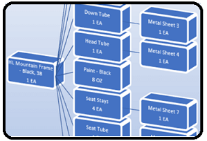
A Hierarchical query is a type of SQL query that is commonly leveraged to produce meaningful results from hierarchical data. Hierarchical data is defined as a set of data items that are related to each other by hierarchical relationships. Hierarchical relationships exist where one item of data is the parent of another item. The real-life examples of the hierarchical data that are commonly stored in databases may include the following:
- Multi-level Bill of Materials (BOM)
- Program call stack
- Employee hierarchy (employee-manager relationships)
- Tasks in a project
- A file system
The Challenge
A membership organization wants to purge old data relating to inactive customers, however due to their data retention policy, they do not want to delete an inactive customer if he/she is related to an active customer. They define "related" as any declared spousal relationships (husband-wife etc..) in the system, plus any secondary relationship (example: ex-spouse, new wife of ex-spouse etc...) Given a table of values that represent current and past spousal relationships, we want to generate list of all "related" customers.
Solution
Use DB2 SQL Hierarchical Query Operators CONNECT_BY_ROOT and CONNECT BY PRIOR, to help us generate a list of relationships.
First, we want to create a table and add sample data.
CREATE TABLE CONJ (SPOUSE1 NUMERIC ( 9, 0) NOT NULL WITH DEFAULT,
                   SPOUSE2 NUMERIC ( 9, 0) NOT NULL WITH DEFAULT)

INSERT INTO CONJ VALUES(1, 2)
INSERT INTO CONJ VALUES(1, 3)
INSERT INTO CONJ VALUES(3, 4)
INSERT INTO CONJ VALUES(5, 4)
INSERT INTO CONJ VALUES(6, 7)
Next, generate list of all relationships:
WITH CONJ2 AS(
  SELECT DISTINCT SPOUSE1, SPOUSE2 FROM conj
  WHERE SPOUSE1 <> SPOUSE2
UNION
  SELECT SPOUSE2, SPOUSE1 FROM conj
  WHERE SPOUSE1 <> SPOUSE2
  ORDER BY SPOUSE1
)
SELECT DISTINCT CONNECT_BY_ROOT SPOUSE1 AS PARENT ,
  SPOUSE2 AS CHILD, LEVEL LEVEL
FROM CONJ2 START WITH SPOUSE1 <> 0
CONNECT BY NOCYCLE PRIOR SPOUSE2 = SPOUSE1
ORDER BY PARENT , CHILD
Output
Note that we pick up the 1-4 relationship (via 1-3, 3-4) and the 3-5 (via 1-3, 4-3, 5-4) relationship.
  PARENT         CHILD
  PARENT         CHILD           LEVEL
     3             4               1
     3             4               3
     3             5               4
     3             5               2
     4             1               2
     4             1               4
     4             2               3
     4             2               5
     4             3               1
     4             3               3
     4             4               2
     4             5               1
     4             5               3
     5             1               3
     5             2               4
     5             3               2
     5             4               1
     5             5               2
     6             6               2
     6             7               1
     7             6               1
     7             7               2
Vocabulary
CONNECT_BY_ROOT is a unary operator that is valid only in hierarchical queries. For every row in the hierarchy, this operator returns the expression for the root ancestor of the row. This operator extends the functionality of the CONNECT BY [PRIOR] condition of hierarchical queries.
CONNECT BY PRIOR In a hierarchical query, one expression in the CONNECT BY condition must be qualified by the PRIOR operator. If the CONNECT BY condition is compound, then only one condition requires the PRIOR operator, although you can have multiple PRIOR conditions. PRIOR evaluates the immediately following expression for the parent row of the current row in a hierarchical query. PRIOR is commonly used when comparing column values with the equality operator. (The PRIOR keyword can be on either side of the operator.) PRIOR causes SQL to use the value of the parent row in the column.
START WITH Use A START WITH clause to specify a root row for the hierarchy. The START WITH clause is not really necessary in this case, but useful if you want to focus your query.
The NOCYCLE clause eliminates cyclic redundance in the queries.
Generating program call documentation
This technique is useful for generating program call structure documentation. If your shop uses X-Analysis or Probe Abstract, you can use this technique to generate call structure documents. Here we iterate through call stack recursively to find programs and files used by program MYPGM. NOCYCLE is used to prevent eliminates cyclic redundances.
SELECT CONNECT_BY_ROOT WHONAM AS TOP_LEVEL, WHONAM AS PARENT , WHRNAM AS CHILD,
   WHRTYP AS Obj_Type, WHRATR OBJ_ATTTR, WHUSG AS USAGE,
LEVEL WHONAM
FROM PROD13109/XDPGREF START WITH WHONAM = 'MYPGM'
CONNECT BY NOCYCLE PRIOR WHRNAM = WHONAM
More on the subject:
Tech tip by Kent Milligan MC press
SQL & Stored Procedures
A stored procedure is a program that can be called to perform specific operations.
Db2 stored procedure support provides a way for an SQL application to define and then call a procedure through SQL statements. Stored Procedures help encapsulate SQL and business logic as they provide reusability and modularity. You may define a procedure as either an SQL procedure or an external procedure. An external procedure can be written in any supported high level language.
Coding stored procedures requires that the user understand the following:
- Stored procedure definition through the CREATE PROCEDURE statement
- Stored procedure invocation through the CALL statement
1. A Stored procedure that adds a record to a table:
-- Create a stored procedure called ADD_CUSTOMER_RECORD
-- this code can be stored in source physical file member SRCFILE(MYLIB/QSQLSRC) SRCMBR(STORED_P1)
-- use RUNSQLSTM to create the stored procedure:
--    QSYS/RUNSQLSTM SRCFILE(MYLIB/QSQLSRC) SRCMBR(STORED_P1)
-- to check that Stored Procedure was created:
--   SELECT SPECIFIC_NAME, SPECIFIC_SCHEMA FROM sysroutines WHERE SPECIFIC_SCHEMA = 'MYLIB'
--  can be run in STRSQL or in SQL client, like the Access Client Solutions Run SQL Scripts Utility
---    CALL  MYLIB.ADD_CUSTOMER_RECORD(1, 'A', 'JOHN DOE', '123 MAIN ST',  5000);

CREATE OR REPLACE PROCEDURE MILIB.ADD_CUSTOMER_RECORD (
    IN P_CUST_CODE INT,
    IN P_CUST_TYPE CHAR(1),
    IN P_CUST_NAME CHAR(25),
    IN P_CUST_ADDRESS CHAR(25),
    IN P_CUST_YR_SALES INT
)
LANGUAGE SQL
BEGIN
    INSERT INTO MYLIB.CUSTOMER (
        CUST_CODE,
        CUST_TYPE,
        CUST_NAME,
        CUST_ADDRESS,
        CUST_YR_SALES
    ) VALUES (
        P_CUST_CODE,
        P_CUST_TYPE,
        P_CUST_NAME,
        P_CUST_ADDRESS,
        P_CUST_YR_SALES
    );
END;
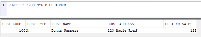
Example of SQLRPGLE program calling a stored procedure with parameters
     // Example of an SQLRPGLE program calling a stored procedure with parameters

     // Declare variables
     Dcl-S P_CUST_CODE Zoned(9:0);
     Dcl-S P_CUST_TYPE Char(1);
     Dcl-S P_CUST_NAME Char(25);
     Dcl-S P_CUST_ADDRESS Char(25);
     Dcl-S P_CUST_YR_SALES Zoned(9:0);

     Eval  P_CUST_CODE = 100;
     Eval  P_CUST_TYPE = 'A' ;
     Eval  P_CUST_NAME = 'Donna Summers';
     Eval  P_CUST_ADDRESS = '123 Maple Road';
     Eval  P_CUST_YR_SALES = 123.45;

     // CAll stored Procedure ADD_CUSTOMER_RECORD
     EXEC SQL CALL ADD_CUSTOMER_RECORD(:P_CUST_CODE,
          :P_CUST_TYPE,
          :P_CUST_NAME,
          :P_CUST_ADDRESS,
          :P_CUST_YR_SALES);

     IF  SQLSTATE = '00000' ;
       // Do something
     ENDIF ;

     Eval *INLR = *ON;
     Return;
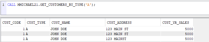
2. A stored procedure to return list of clients based on client type
-- Stored Procedure to return list of clients based on client type
-- source can be stored in SRCFILE(MYLIB/QSQLSRC) SRCMBR(STORED_P2)
-- to create stored procedure:
--   QSYS/RUNSQLSTM SRCFILE(MYLIB/QSQLSRC) SRCMBR(STORED_P2) COMMIT(*NONE)
-- run in SQL client (like the Access Client Solutions Run SQL Scripts Utility)
---  CALL MYLIB.GET_CUSTOMERS_BY_TYPE('A');

CREATE OR REPLACE PROCEDURE
      MYLIB.GET_CUSTOMERS_BY_TYPE (IN P_CUST_TYPE CHAR(1))
LANGUAGE SQL
RESULT SETS 1
BEGIN
    -- Declare a cursor to fetch the matching customers
    DECLARE CUST_CURSOR CURSOR WITH RETURN FOR
    SELECT CUST_CODE, CUST_TYPE, CUST_NAME, CUST_ADDRESS, CUST_YR_SALES
    FROM MYLIB.CUSTOMER
    WHERE CUST_TYPE = P_CUST_TYPE;

    -- Open the cursor
    OPEN CUST_CURSOR;
END;